This article is mentioned in:

Introduction

Colorectal cancer (CRC) ranks among the three most common types of cancer in terms of both incidence and cancer-associated mortality in Western industrialized countries (1). Each year nearly 1.3 million new cases of CRC are reported, and ~700,000 patients succumb to the disease worldwide (2). The lifetime risk of developing CRC may reach 6% of the population living in developed countries (3,4). CRC ranks highest in incidence rates in Europe, second only to lung cancer, and it causes ~204,000 deaths every year (5). The age-specific incidence of CRC rises sharply after 35 years of age, with ~90% of cases occurring in persons >50 years of age (6). As in other developed areas, in Italy, the incidence rate of CRC ranks third highest for men (after prostate and lung cancer), and second for women (after breast cancer) (7). The burden of the disease, however, remains a serious concern in Italy as well as worldwide, due to the social impact, costs and rates of mortality (8). According to the theory by Vogelstein, CRC progresses through three precisely-connected stages: Initiation, a process that modifies the molecular message of the normal cell; promotion, in which signal transduction cascades are altered; and progression, which involves phenotypically-altered, transformed cells (9). The first morphological changes observed in the progression of CRC are represented by the formation of aberrant crypt foci (ACF). The most striking feature of the ACF is the shape of the gland lumen, which is considerably modified when compared with the normal mucosa, and strongly dependent on the histological structure (10). Furthermore, the phenotypic and genotypic characteristics of ACF are different from those of normal crypts. These characteristics were first described by Bird in mice exposed to azoxymethane, and were subsequently studied extensively in humans by Roncucci (11,12). Currently, it is impossible to identify the ACF via routine colonoscopy; however, in humans, the presence of ACF is identifiable via the use of high-resolution chromoendoscopy with the aid of particular dyes, such as methylene blue or indigo carmine (13). A previous study reported that ACF occurs sporadically between 40 and 45 years of age, when predominantly single foci are observed (14). After 45 years, the number of ACF rapidly increases to reach the plateau phase at ~60 years of age, and slowly decreases thereafter. Other studies have reported similar incidence rates of ACF in these age brackets (15,16). It is essential to identify and remove these early lesions for an adequate CRC prevention strategy (17). Furthermore, accurate tumor grading is necessary for patient survival and can be achieved most effectively in stained histopathological sections harvested via biopsy or during surgery. Medical databases are fundamental in the development of new techniques for early detection of neoplastic cells. They are, however, difficult to obtain, since the labeling of the images is often operator-dependent and requires specialized skills. The considerable complexity and quantity of the structures present in the biological tissue represents a fascinating challenge for pathologists both in manual and automatic analyses of histopathological slides. Although certain studies have presented a reasonable consensus among experienced pathologists and satisfactory results on their intra-observer reliability, other studies have stated that even experienced pathologists often disagree on tissue classification. Therefore, the use of expert scores as a gold standard for histopathological examination could lead to inappropriate evaluations (18–20). In addition, quantitative characterization of pathology imagery is important not only for clinical applications but also for research applications. Recent studies have proven that the deep learning (DL) approach is superior for tasks of classification and segmentation on histological whole-slide images, as compared with the previous image processing techniques (21–23). As examples, DL models have been developed to detect metastatic breast cancer (24), to identify mitotically active cells (25), to identify basal cell carcinoma (26) and to grade brain gliomas (27) using hematoxylin and eosin (H&E)-stained images. Histopathological sections of colon tissues, stained with H&E representative of the adenoma-carcinoma sequence are presented in Fig. 1.

Figure 1. Neural network comprising four modules, each consisting of Convolution (3×3 kernels with 1pixel padding), BatchNorm2d, RELU and Maxpool, followed by a flattening operator, and 3 linear modules consisting of Linear, RELU and BatchNorm1d; RELU, rectified linear unit.

DL techniques for image recognition have proven extremely effective in a broad number of applications, often surpassing human performances. The general idea is that a sufficiently flexible software network can be trained, i.e., values can be assigned to its parameters, in order to recognize images by examining a broad set of labeled images. Once trained, the network can be used on unlabeled images to assign the correct corresponding label.

Although the field is still rapidly evolving, some general features of the network structure required to perform a given task are sufficiently understood, meaning that the primary obstacle for new applications is the lack of labeled training sets.

Several applications of DL techniques to classify colorectal cells have been published. A summary of the approaches used is reported in the GLAS challenge contest summary (28). By the very nature of the challenge, these methods are based on segmentation, i.e., individual pixel labeling (29), which is an effective and sensible approach from a computational perspective, but requires significant investment in preparing a training set where each individual pixels is assigned by human inspection to a given part of the cell or the background. In addition, it is not clear how the trained networks would perform on images obtained with different instruments and resolutions. As the quality of colorectal tissue images is instrument-dependent and tends to improve over time as new microscopes replace older models, this last point is particularly relevant.

The aim of the present study was to use a DL algorithm to classify images of colorectal tissues that bypasses segmentation and labels the raw image directly. Thus, the method used in the present study did not rely on a segmented training set, but rather on the readily available labeled images, as routinely found in a pathologist report. Hence, the network created in the present study can be easily retrained whenever the quality of the images changes, with minimal human effort.

In addition, a more articulate classification was performed in the present study; instead of two labels (benign and malignant), four categories were employed (normal, preneoplastic, adenoma and cancer) representing the disease progression. On the one hand, this implied more uncertainty in the labeling, as images for neighboring categories may appear similar and a trained pathologist would rely also on other information and/or a collection of several images to provide a diagnosis. On the other hand, the ability to recognize the different stages of cancer development will prove extremely valuable in providing more specific diagnoses and eventually early treatments.

In the present study highly accurate and reproducible results were obtained from biomedical image analysis (overall accuracy, >95%), with the potential to significantly improve both the quality and speed of medical diagnoses. The present study also states the performance level of the DL algorithm on the GLAS challenge images. Although no patent should be based on this work without explicit written consent from the authors, the algorithm used is not proprietary and other researchers are invited to share it for testing purposes.

Materials and methods

Patients and samples

The database used in the present study consisted of 393 images, divided into the 4 categories or labels: Normal mucosa (m), preneoplastic lesion (ACF) (p), adenoma (a) and colon cancer (k). All images were obtained from patients who underwent primary surgery or colonoscopy at the Modena University Hospital between 1998–2008. Normal mucosa images were obtained from 44 patients, preneoplastic lesions (ACF) from 45 patients, adenoma images from 76 patients, and colon cancer tissue images from 58 patients diagnosed with CRC. The present study was granted ethical approval by the local operative ethics committee of the Policlinico Hospital of Modena. Written informed consent was not required, since the present study was retrospective in design and the amount of specimens obtained was extensive. Tissue images were stained with haematoxylin and eosin (H&E) and digitized with an optical microscope Leica IRBE with CCD Rising Tech. Sony CCD Sensor (USB2.0 5.0MP CCD ICX452AQ) camera and Software Image Pro Plus (v4.5). Images were captured under ×20 magnification and a resolution of 600 dpi. Slides were scanned using a unique study ID and without identifiable data linked to the patient. In the present study, two pathologists from the Unit of Pathology of Modena, and Bologna independently reviewed the whole-slide images in the training and test datasets in order to identify the type of colorectal lesions as reference standards. When disagreements regarding the image classification occurred, the pathologists resolved the issue through further discussions. When it was not possible to reach a consensus on a lesion type for an image, that image was discarded and replaced by a new one in order to maintain accuracy.

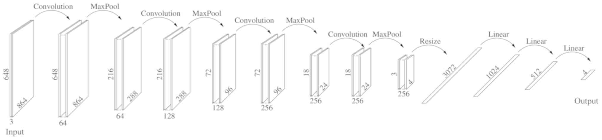
Dataset and the DL algorithm

The present study divided each image in the database into 9 subimages, each 864×648 pixels, and relabeled each one individually, discarding those not recognizable, resulting in a final dataset containing 2,513 images. Disjoint subsets were then randomly created the: Training (2,012 images), validation (251 images) and test (250 images). Each of the given sets was further divided into the label categories reported in Table I. This was referred to as the Small Dataset. A Large Dataset was also created as follows: Each image, within the corresponding subset, was rotated 180 degrees, and reflected along both the vertical and horizontal axes, in order to obtain a dataset four times larger, i.e., comprising 10,052 images (Table I). The DL algorithm created in the present study was implemented on the Pytorch platform with hardware Nvidia Titan XP and Quadro P6000 and consisted of the sequences reported in Fig. 1.

Table I. Small dataset and large dataset.

Table I.

Small dataset and large dataset.

A, Small dataset
Small Dataset	Normal mucosa	Preneoplastic lesion	Adenoma	Colon cancer	Total
Training	404	407	685	534	2,012
Validation	50	51	86	64	251
Test	50	51	85	64	250
B, Large dataset
	Normal mucosa	Preneoplastic lesion	Adenoma	Colon cancer	Total
Training	1,616	1,628	2,736	2,068	8,048
Validation	200	204	344	256	1,004
Test	200	204	340	256	1,000

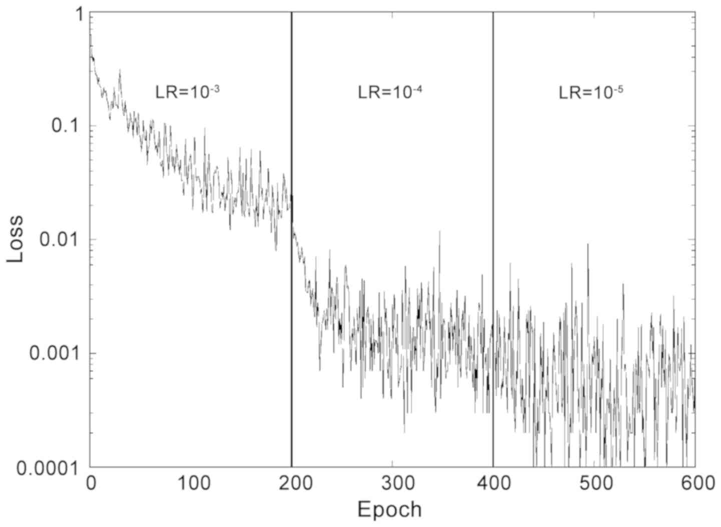
Given the relatively small training set, a small batch size, consisting of 10 images was selected. During the validation, performed initially using the Small Dataset, the optimizer Adam was selected over SGD and Adagrad, which provided slightly worse levels of accuracy (−5%). For the loss function calculation, the present study opted for Softmax. The weight decay was set to 10−5 and cycles of 200 epochs were performed with different learning rates. A short training of two cycles was used, with learning rates of 10-3 and 10−4, respectively, and a long training, which included a third cycle with a learning rate 10−5. The loss function during training is reported in Fig. 2. During training, each epoch runs in ~58 sec (Small Dataset) or 3.50 min (Large Dataset), so the complete training is completed in <10 (Small) or 40 (Large) hours on this system. Evaluation of the test set took ~10−2 sec/image, making this Neural Network practical for fast screening of thousands of images in seconds. In order to estimate the stability of the optimized network, after the aforementioned training, the present study performed 10 evaluations of the test set separated by 4 epochs of further training. The accuracies are reported as the average value from these 10 evaluations, and the standard deviation was used as an estimate of the uncertainty. The same procedure was followed for a number of optimizations starting from scratch and using different partitions of the original image dataset and different weights for the Adam optimizer. It was observed that the accuracies were generally within two standard deviations of each other.

Figure 2. Logarithmic plot of loss-of-function during typical optimization.

Results

The accuracy of the test set following the Short and Long trainings is presented in Table II. The present study also measured the accuracy for the nearest match. Accuracies, expressed as a percentage of correct results ± standard deviation, were computed for the test set using different optimization and evaluation conditions. Short training indicates 200 epochs with learning rate 10−3 and 200 epochs with learning rate 10−4. Long training adds another 200 epochs with learning rate 10−5. For the exact match, predictions were considered correct only if they matched the target exactly. In the nearest match, neighboring labels were also regarded as correct, as described later. The Small Dataset refers to the original 2,513 images divided into training, validation and test sets. The Large Dataset also includes rotations and reflections, for a total of 10,052 images. For normal mucosa (m) the nearest match is the preneoplastic lesion (p); for (p), they are (m) and (a) the adenoma; for (a), they are (p) and (k) cancer; while for (k) is just (a). Representative histological images of the aforementioned categories are presented in Fig. 3, and these four images were all correctly labeled by the DL algorithm.

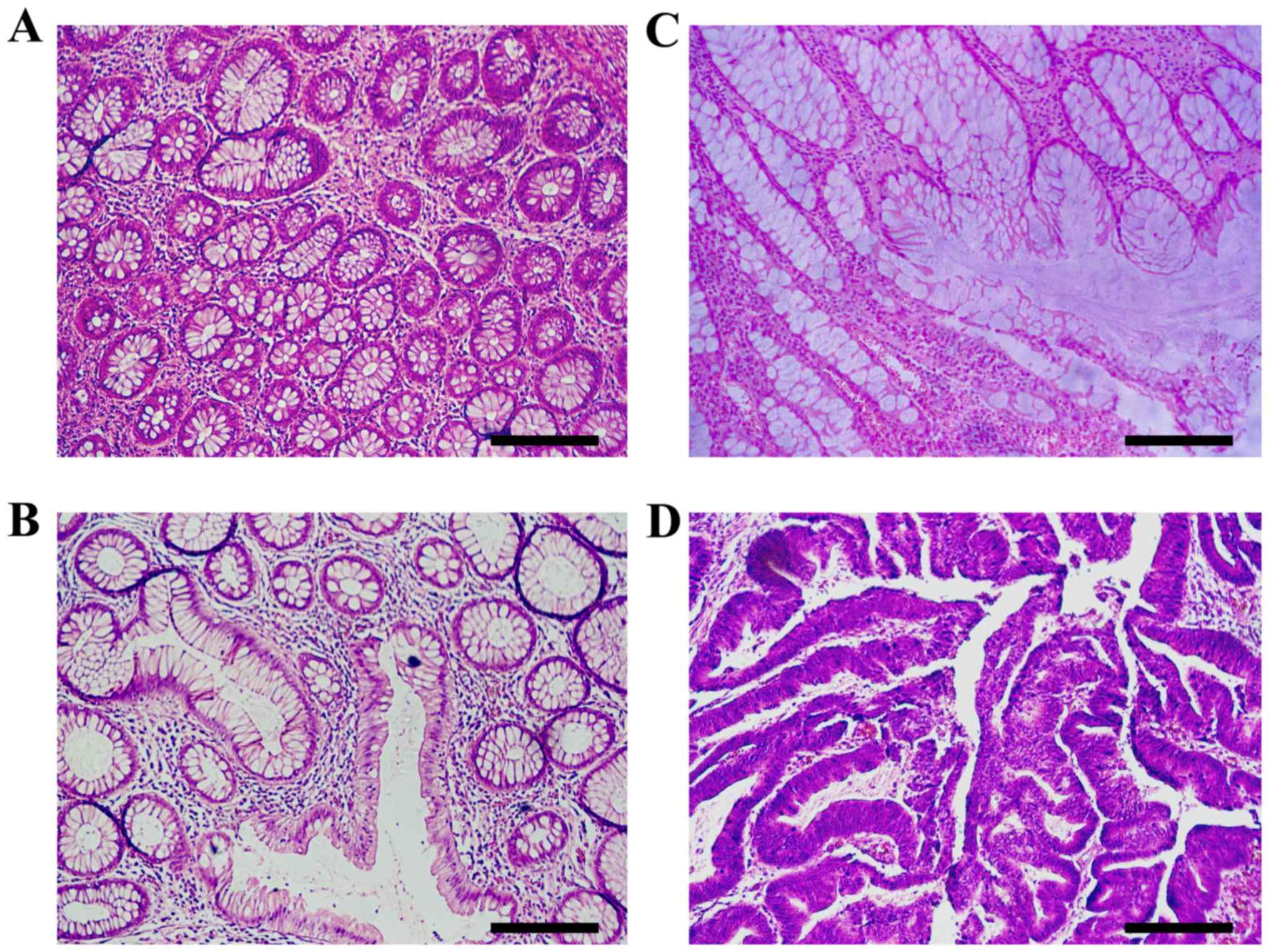Figure 3. Histopathological sections of hematoxylin and eosin stained colon tissues that are representative of colorectal carcinogenesis. (A) Normal mucosa exhibits benign glands consisting of a regular circular lumen in cross section. (B) Pre-neoplastic lesion (aberrant crypt foci) consists of larger glands with enlarged epithelial nuclei, often stratified and crowded. (C) Adenoma is characterized by ovoid enlarged nuclei, vesicular dispersed chromatin and occasional mitoses. Sections exhibit an uneven distribution of goblet cells within crypts, luminal serration, budding, branching, crowding and fusion of glands. (D) In carcinoma, architectural changes increase with evolution and progression of malignancy. Luminal serration, budding, branching, crowding and fusion of glands are presented. Scale bar, 210 µm.

Table II. Test accuracy after short and long training.

Table II.

Test accuracy after short and long training.

Training	Exact match large dataset (%)	Nearest match large dataset (%)	Exact match small dataset (%)	Nearest match small dataset (%)
Short	93.79±0.76	99.85±0.11	92.92±0.86	99.20±0.25
Long	95.28±0.19	99.90±0.00	93.08±0.57	99.20±0.00

[i] Accuracies for the test set of different optimization and evaluation conditions are expressed as the percentage of correct results ± standard deviation.

The GLAS challenge dataset (29,30) was used to further validate the approach of the present study against drastically different images. All images from the GLAS training were considered, including test A and test B sets combined. These differ from those of the present study: Both sets refer to ×20 magnification, but the images used in the present study were collected with a resolution of 0.426 mm/pixel, vs. 0.620 mm/pixel in the GLAS dataset. They were also different sizes. Hence, each GLAS image was expanded by bicubic interpolation by a factor of 0.620/0.426 in order to achieve the same nominal resolution as that in the present study. Of course, this introduces some blurring and the quality of the resulting images was different from that used for training. Each of the GLAS images were then cropped to 864×648 pixels. Of the 165 GLAS images, 14 were discarded, as they were too small. The majority of the remaining 151 were then cropped to focus on the central part of the image. A few cases comprising significant portions of non-tissue background were cropped close to one edge or corner in order to include as much tissue as possible.

Discussion

Researchers both in the image analysis and pathology fields have recognized the importance of quantitative analysis of pathology images. The current pathological diagnosis is based on a detailed and careful observation of the abnormal morphological changes, and is based on specific and precise criteria. However, it is a subjective, though educated opinion. Thus, the need for a quantitative assessment based on slide images of digital pathology is urgently required. This quantitative analysis of digital pathology is important not only from the diagnostic point of view, but also to understand the reasons that led to a specific diagnosis (for example, the altered size of the lumen glands of the Lieberkuhn crypts, indicating a potential malignant hyperplasia). Furthermore, the quantitative characterization of pathological images is important both for clinical applications (e.g., to decrease/eliminate inter- and intra-observer variations in diagnosis) and for research applications (e.g., to understand the biological mechanisms underlying the pathological process). From a histopathological perspective, the crypts of the Lieberkuhn have different characterizing components, including the lumen, epithelial cells and stroma (connective tissue, blood vessels, nervous tissue, etc.). The epithelial cells form the outline of the gland, which encloses the cytoplasm and the lumen, while the stroma is not considered part of the gland. If only non-cancerous (benign) glands are considered, the DL algorithms must actually be able to manage and recognize a significant variability of shape, size, position, consistency and staining of the glands. Obviously, when the analysis is performed on the cancerous tissue, the glands appear significantly different from the benign glands, and the presence of artefacts or corrupted areas further aggravates the problem. Therefore, machine learning approaches are primarily used to develop extremely precise models trained with labelled examples that can address the problematic tissue variability. An effective algorithm for medical diagnoses requires large training datasets, which, in general, are extremely difficult to obtain, in order to correctly classify the different features of benign and malignant gland types (Fig. 3). Colorectal carcinogenesis is a multi-step process characterized by marked morphological changes. The normal epithelium becomes a hyperproliferative mucosa and subsequently gives rise to a benign adenoma, which can then progress into carcinoma and metastases (9). Furthermore, CRC presents an intratumor heterogeneity highlighted by genetic analysis (31). From the reported accuracies, it was observed in the present study that the Large Dataset generally provided better results than the Small Dataset. Thus, as previously reported (28,29), including the same image with different orientations is a viable strategy to improve the dataset. In the present study, the transformed images were placed in the same set (training, validation or test) as the original so as to not bias the results by including the same image in the test set as was used in training, with a different orientation. The effect of a total randomization of the Large Dataset was also tested, and although the performance was slightly improved, the differences were within two standard deviations. The reported results also indicated that the last 200 epochs in the Long training time had a small effect on the loss. This seemed to improve the accuracy for the exact match, but not for the neighboring match. Although from Table I it appears that the standard deviation was significantly smaller after the Long training, this effect was largely due to the 10 samples used to compute the average and standard deviation being separated by 4 epochs of training. The learning rate for this extra training was 10−4 after the Short optimization, but it was 10 times smaller after the Long one. Since the parameters change was tied to the learning rate, the sets of parameters used for the 10 cases after the Long optimization were more similar to each other than those after the Short optimization, hence they provided more similar classifications. Thus, a direct comparison of standard deviations is only meaningful when the same learning rate is used. In the present study, this effect was tested by increasing the learning rate or the number of epochs between evaluations after the Long training, and revealed that this was indeed the case. This also indicates that there is an association between the 10 evaluations after the Long training, so the present study recommends using the standard deviation from the Short training to estimate the uncertainty. The results for the Long training and Large Dataset are detailed in the confusion matrix in Table III, where percentages are presented as averages over the 10 measures. In this case, only 1 of the 1,006 test cases falls outside the nearest neighbor range. When repeating the optimization it was typically observed that this number was between 0 and 2. The accuracy for exact matches was close to 95%, making the procedure attractive for clinical use. In addition, when the nearest cases were included, it surpassed 99.8%, indicating that most mislabeling refer to one of the nearest neighbors. As mentioned in the ‘Introduction’ of the present study, when using four labels, this kind of mislabeling would not be unusual even for trained pathologists. Finally, the reported DL network structure derives from several attempts where different numbers and sizes of hidden layers were used. Although efforts were made to maximize the accuracy on the validation set, it is still possible that modifications of the network used in the present study may improve the performance. To the best of our knowledge, there are currently no alternative methods for automatic classification into the four key categories of colorectal tissue images based on the approach that is proposed in the present study. A comparison can be attempted with the GLAS Challenge contest (28), although the aim there was segmentation and classification based on only two categories. Furthermore, accuracies were based on individual pixels and segmented objects, and were between 80–90%, significantly lower than the ones obtained in the present study. To this end, the present study processed the GLAS dataset as described in the previous section, obtaining images that are comparable to those in the present study, but with a different resolution. As the GLAS challenge only has two categories (benign and malignant), three of the four categories (preneoplastic, adenoma and cancer) were grouped as malignant, leaving the fourth (normal mucosa) as benign. The same evaluation as in the test of the present study, i.e., 10 evaluations separated by 10 training epochs, yields an accuracy of 81.7 with standard deviation 1.1. This accuracy is smaller than those obtained by some GLAS challenge participants (29). However, considering that the network training is based on images obtained with different instruments and resolution, and that the classification scheme is not the same, it demonstrates that the approach used in the present study is viable and could be exported to broader datasets, provided enough diversity is included in the training set. This result also indicates that networks trained on images from a given microscope model may not perform as well on images from another one, making the unsegmented approach of the present study more appealing for easy adjustments. The fact that our approach is fundamentally different from those used in the GLAS challenge should be noted, as it is not based on segmentation and recognition of individual features, but rather on direct classification from raw images.

Table III. Confusion matrix for long training and large dataset. Rows correspond to predictions, columns to true labels.

Table III.

Confusion matrix for long training and large dataset. Rows correspond to predictions, columns to true labels.

True→ Predicted↓	M	P	A	K	Precision False positive
M	18.2	0.3	0.0	0.0	98.2 1.8
P	1.9	18.3	0.8	0.0	87.3 12.7
A	0.0	1.5	33.1	0.0	95.6 4.4
K	0.0	0.1	0.8	25.6	99.3 0.7
Recall False negative	90.7 9.3	90.3 9.7	97.4 2.6	100.0 0.0	95.34.7

[i] Rows correspond to predictions, columns to true labels. Each box contains the percentage with respect to all 1,006 test cases. The diagonal (bold) data contains correct predictions, all other data contains mislabeling. Bottom right box indicates the overall precision end error. M, normal mucosa; P, preneoplastic; K, cancer; A, adenoma.

The results from the present study suggest the potential for this method to become of practical assistance to pathologists.

In conclusion, the present study collected a microscope image database of human colorectal tissue, including normal mucosa, preneoplastic lesion, adenoma and carcinoma. The DL algorithm used in the present study, trained on part of the dataset, was able to correctly assign >95% of the test cases, and the majority of the mislabeled images were assigned to neighboring categories. The results from the present study suggest that DL techniques may provide a valuable tool to assist human operators for histological classification of the different steps of the adenoma-carcinoma sequence, typical of colorectal tumors.

Acknowledgements

The authors would like to Dr Alessandro Achille and Dr Patrik Chaudhari (UCLA) for their helpful comments.

Funding

NVIDIA Corporation (Santa Clara, USA) provided Titan XP and a Quadro P6000 graphic processing unit through their GPU grant for research purposes. Marie Slodova Curie Action funded the current study via the GHAIA Geometric Harmonic Analysis for Intersciplinary Application (grant no. GA 777822).

Availability of data and materials

The datasets used and/or analyzed during the present study are available from the corresponding author on reasonable request.

Authors' contributions

PS, RF and FF conceived and designed the present study. PS, LL and LR acquired the data. PS, LL, LR and RF analyzed and interpreted the data. RF, FF and GF implemented the Neural network. LL and LR critically revised the manuscript. PS, RF and FF wrote the manuscript.

Ethics approval and consent to participate

The present study was granted approved by the local Operative Ethics Committee of The Policlinico Hospital of Modena.

Patient consent for publication

All patients provided written informed consent for the publication of any associated data and accompanying images.

Competing interests

The authors declare that they have no competing interests.

References